Table Of Content
For example, you can combine a column or area chart with a line chart to present dissimilar data, for instance an overall revenue and the number of items sold. When the chart options pop up — either on the ribbon or under your cursor if you right-clicked — you’ll next click Change Chart Type. A menu will pop up with a variety of chart type options on the left.
Chart Mistake 1: Redundant Information using PowerPoint or Excel Charts
After you input your data and select the cell range, you’re ready to choose the chart type. In this example, we’ll create a clustered column chart from the data we used in the previous section. For more chart types, click the More Column Charts… link at the bottom.
Step 12: Delete a Chart
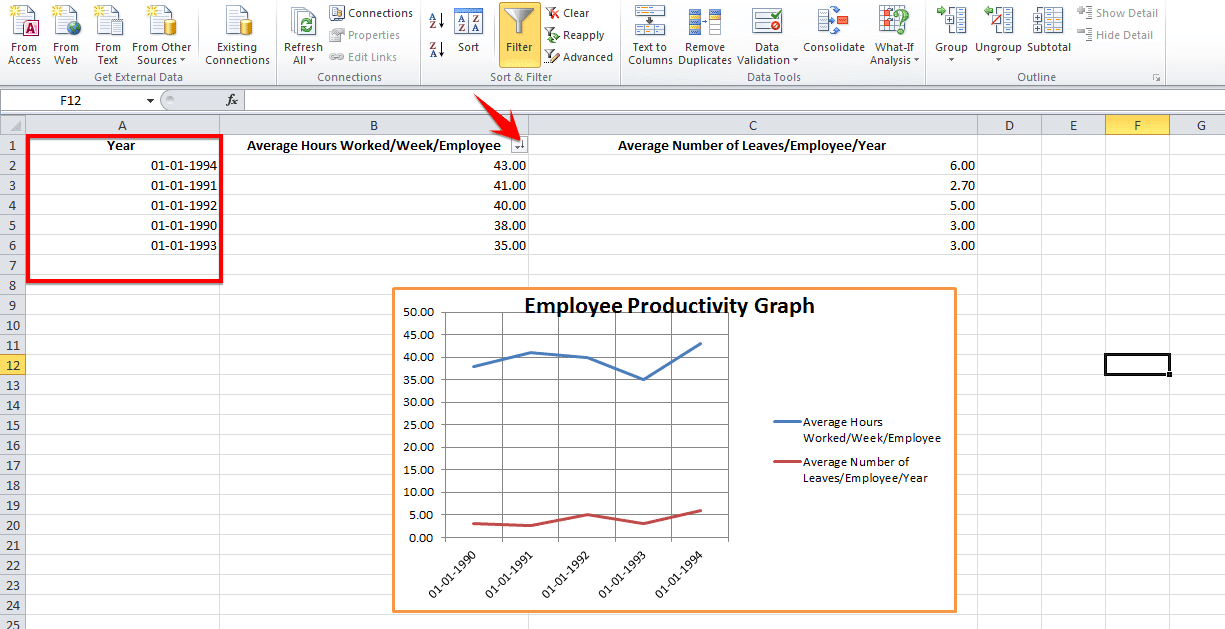
In this example, we are going to make a graph based on the following table. One common mistake is trying to cram too much information into a single graph. While it may be tempting to include every data point and trend, doing so can make the graph cluttered and difficult to interpret. Instead, focus on the most relevant and important data points that support your analysis. To save your Excel graph as a photo, right-click on the graph and select Save as Picture. Right after making your chart, the title that appears will likely be “Chart Title” or something similar, depending on the version of Excel you‘re using.
Adding a Chart Title
I can help with advice if needed (contact me via the infoDiagram contact page). The next trap people fall into when presenting data is selecting low-contrast color schemes. High-contrast colors ensure that all elements of the chart are easily discernible, enhancing the overall readability. WPS Excel Graph Templates is a collection of striking graph templates meant to enhance data visualization. Each template comes equipped with a short tutorial that guides you on how to exploit the template’s full potential.
Choose from the graph and chart options.
To change the color theme of your Excel graph, click the Chart Styles button, switch to the Color tab and select one of the available color themes. Your choice will be immediately reflected in the chart, so you can decide whether it will look well in new colors. To change the legend's formatting, you have plenty of different options on the Fill & Line and Effects tabs on the Format Legend pane. Microsoft Excel automatically determines the minimum and maximum scale values as well as the scale interval for the vertical axis based on the data included in the chart. However, you can customize the vertical axis scale to better meet your needs. To add a chart title in Excel 2010 and earlier versions, execute the following steps.
To take your Excel dashboard to the next level, consider incorporating slicers. Slicers are interactive filters that allow users to dynamically segment and explore the data presented in your pivot tables and charts. By clicking on different slicer options, users can instantly update the dashboard to display only the data that meets their selected criteria.
How to Find and Use Excel's Free Flowchart Templates - Lifewire
How to Find and Use Excel's Free Flowchart Templates.
Posted: Mon, 26 Sep 2022 07:00:00 GMT [source]
3) This will adjust the chart so that the tasks are displayed in the desired order. Follow these steps to effectively manage and visualise multiple projects using a Gantt chart in Excel. Right click on the horizontal axis in your chart and select Format Axis… in the context menu.
How to Make a Graph in Google Sheets - Lifewire
How to Make a Graph in Google Sheets.
Posted: Mon, 01 Nov 2021 07:00:00 GMT [source]
Let's start by introducing our Excel worksheet so you understand what we aim to achieve with this blog. Alternatively, you can right-click anywhere within the graph and select Change Chart Type… from the context menu. Click the arrow next to Axis, and then click More options… This will bring up the Format Axis pane. Or, you can click the Chart Elements button in the upper-right corner of the graph, and put a tick in the Chart Title checkbox. His writing has appeared on dozens of different websites and been read over 50 million times. The first thing you need to do is select the data you want to include in your graph.
By mastering the art of creating interactive Excel dashboards, you’ll be well-equipped to drive sales performance and achieve your business goals. So dive in, experiment with different techniques, and unlock the full potential of your sales data today! For more help and support on using Microsoft products jump over to the official Microsoft support website. Small touches like consistent formatting, clear labeling, and intuitive navigation can go a long way in making your dashboard more engaging and user-friendly.
There are many types of graphs available in Excel, such as column, line, pie, bar, area, scatter, and more. Think about what makes the most sense for the data you’re working with and the story you’re trying to tell. Legends tell you information you can read easily on the graph. If you have a ton of X-axis categories or multiple data points per category, then using legends makes sense.
As you can see in the picture below, the left chart contains information about data value – the CAPEX last year versus the budgeted value – in two places. It’s enough to keep only one of them for sake of data visualization clarity. The following step-by-step example shows how to create a semi-log graph in Excel for a given dataset. When it comes to the needs of business professionals, HubSpot provides templates that align well with various business data presentation requirements. Specialized chart requirements, like organizing charts, can be met with platforms such as Pingboard and Smartsheet.

Sometimes, data showing meaningful change is still within normal parameters. Sometimes, what seems like a slight difference is significant. This can help you understand which products sell well in different geographies during the same time frame.
This automatically inserts a new chart based on whatever type is set as default. Whenever you insert or select a chart, you’ll notice additional Chart Tools appear on the ribbon, divided into Chart Design and Format tabs. To customize your graph, you can follow the same steps explained in the previous section. All functionality for creating a chart remains the same when creating a graph. In the following section, we’ll walk you through the specifics of creating a clustered column chart in Excel 2016. When you create a graph in Excel, it is automatically embedded on the same worksheet as the source data.
In the video, I’ll walk you through creating a graph using a sample dataset. For cluster column charts, there are 14 chart styles available. Excel will default to Style 1, but you can select any of the other styles to change the chart appearance. Use the arrow on the right of the image bar to view other options. Charts and graphs in Microsoft Excel provide a method to visualize numeric data.
Notice how much easier it is to interpret the y values in this graph compared to the previous graph. The x-axis remains on a linear scale, but the y-axis has been converted into a logarithmic scale. 3) Afterwards, form the Format Data Series, select 3-D Format, and choose Angle type bevel from the Top Bevel drop-down. 1) From the Format Data Series task pane, click on any of the red bars. We're going to show you how you can successfully create a Gantt Chart for Multiple Projects in Excel.
Follow the steps below to learn how to chart data in Excel 2016. To apply the chart template to an existing graph, right click on the graph and choose Change Chart Type from the context menu. Or, go to the Design tab and click Change Chart Type in the Type group. If you are really happy with the chart you've just created, you can save it as a chart template (.crtx file) and then apply that template to other graphs you make in Excel. The most recent versions of Microsoft Excel introduced many improvements in chart features and added a new way to access the chart formatting options. If you want to compare different data types in your Excel graph, creating a combo chart is the right way to go.


No comments:
Post a Comment